Linz post-processing examples

import os
import pandas as pd
import toto
from toto.inputs.linz import LINZfile
from toto.core.totoframe import TotoFrame
from toto.filters.despike_phasespace3d import despike_phasespace3d
from toto.filters.lanczos_filter import lanczos_filter
from toto.filters.detrend import detrend
import numpy as np
import matplotlib.pyplot as plt
import requests
import zipfile
import datetime
import copy

Link to lINZ files

BASEURL='https://sealevel-data.linz.govt.nz/tidegauge/%s/%i/%i/%s_%i_%s.zip'
#BASEURL='https://sealevel-data.linz.govt.nz/tidegauge/AUCT/2009/40/AUCT_40_2009085.zip

Station to download

tstart=datetime.datetime(2019,1,1)
tend=datetime.datetime(2020,1,1)
station='AUCT'
sensor=40

if not os.path.isfile('AUCT_40_2019001.csv'):
    # Download Linz elevation file from `tstart` to `tend` at `station` tidal gauge
    dt=copy.deepcopy(tstart)
    files=[]
    while dt<tend:
        fileout='%s_%03i.zip' % (station,dt.timetuple().tm_yday)
        linzurl=BASEURL % (station,dt.year,sensor,station,sensor,str(dt.year)+'%03i'%dt.timetuple().tm_yday)
        linzfile = requests.get(linzurl, allow_redirects=True)
        if linzfile.status_code != 404:
            files.append(fileout)
            with open(fileout, 'wb') as fd:
                for chunk in linzfile.iter_content(chunk_size=128):
                    fd.write(chunk)
        dt+=datetime.timedelta(days=1)

    #%%
    # Download AUCKLAND station README
    fileout='%s_readme.txt' % station
    linzurl='https://sealevel-data.linz.govt.nz/tidegauge/%s/%s_readme.txt' % (station,station)
    linzfile = requests.get(linzurl, allow_redirects=True)
    with open(fileout, 'wb') as fd:
        fd.write(linzfile.content)

    #%%
    # Unzip the all files and save to file
    filenames=[]
    for file in files:
        with zipfile.ZipFile(file) as z:
            filenames.append(z.namelist()[0])
            z.extractall()

    #%%
    # Merge all timeseries into 1
    with open(filenames[0], 'w') as outfile:
        for fname in filenames[1:]:
            with open(fname) as infile:
                outfile.write(infile.read())

Reading the files into a dataframe df=LINZfile(filenames[0])._toDataFrame()[0]

df=LINZfile('AUCT_40_2019001.csv')._toDataFrame()[0]

Out:

Line SUMMARY OF TIDE GAUGE ZERO not found

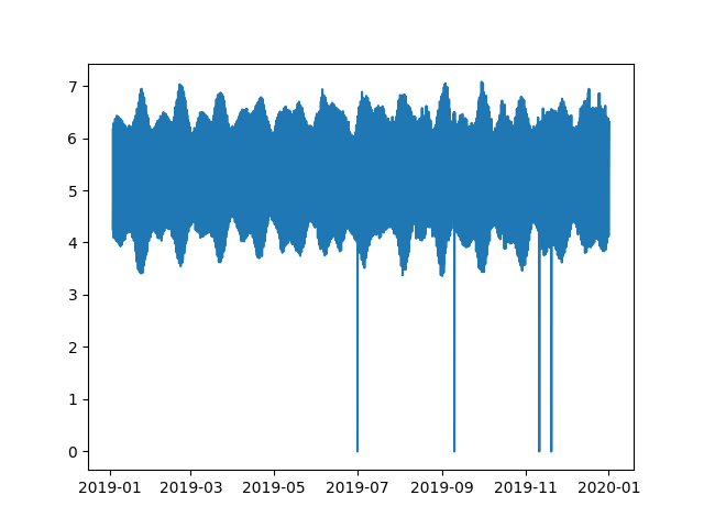
plot the raw timeseries

df.rename(columns={'elev'+str(sensor):'elev'},inplace=True)
plt.plot(df.index,df['elev'])
plt.show(block=False)

Add the Panda Dataframe to a Totoframe. The reason is so if anyhting changes to the dataframe, the metadata get saved in a sperate dictionary. Also the dataframe gets clean and any gaps in the data get filled with NaN. The timeserie is now with a uniform time interval

tf=TotoFrame()
tf.add_dataframe([df],[station])
df=tf[list(tf.keys())[0]]['dataframe']

Resample to hourly otherwise the next steps might crash

df = df.resample('1H').nearest()

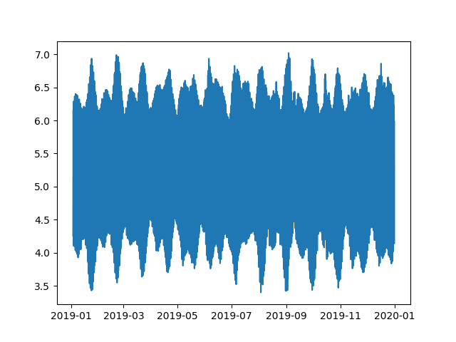
Apply a phase-space method filter to remove most of the spike

df['filtered']=despike_phasespace3d(df['elev'])
plt.plot(df.index,df['filtered'])
plt.show(block=False)

Remove the rest of the spike if needed

Now the timeseries is clean will start extracting the component

del df['elev']
df.rename(columns={'filtered':'elev'},inplace=True)

Detrending but don’t think there is much to detrend Before detrending we store the position of all the gaps

f = np.where(np.isnan(df.elev.values) == 1)
# We fill gaps using the mean
df.fillna(df.elev.mean(), inplace=True)
# Get the detrended time series
df['et'] = detrend(df['elev'],args={'Type':'linear'})
# Strore the trend
df['trend'] = df['elev']-df['et']

the tidal analysis

lat=tf[list(tf.keys())[0]]['latitude']
tmp=df.TideAnalysis.detide(mag='et',\
                                args={'minimum SNR':2,\
                                      'latitude':lat,
                                      'constit': 'auto'
                                     })

df['tide']=tmp['ett'].copy()
# Replace the gap filled data with tidal elevation
df['et'].values[f] = df['tide'].values[f]

Out:

solve: matrix prep ... solution ... diagnostics ... done.
prep/calcs ... done.

Monthly sea level analysis using lanczos filter

df['msea'] = lanczos_filter(df['et'], args={'window':24*30,'Type':'lanczos lowpas 2nd order'})

# We subtract that component to what is left of the signal
df['et'] = df['et'] - df['msea']

Storm surgeanalysis using lanczos filter

df['ss'] = lanczos_filter(df['et'], args={'window':40,
    'Type':'lanczos lowpas 2nd order'})
# We subtract that component to what is left of the signal and get the residual
df['et'] = df['et'] - df['ss']

Finally we subtract the tide to get the residual

df['res'] = df['et'] = df['et'] - df['tide']

for key in df.keys():
    if key!='time':
        df[key].values[f] = np.nan

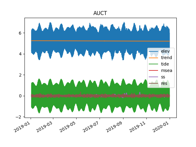
Plot the results

fig = plt.figure()
ax=plt.subplot(111)
plt.title(station)
variables_to_plot=['elev','trend','tide','msea','ss','res']
for v in variables_to_plot:
    plt.plot(df.index,df[v],label=v)


plt.legend()
fig.autofmt_xdate()
plt.show(block=False)

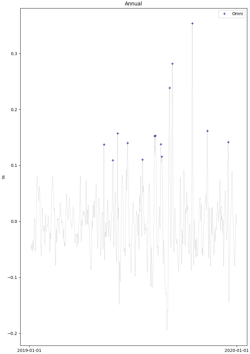
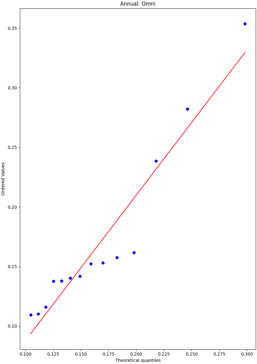
Water elevation fit the distribution

df.Extreme.distribution_shape(mag='ss',\
        args={'Fitting distribution':'Weibull',#'Weibull','Gumbel','GPD','GEV'
         'method':'ml',#'pkd','pwm','mom', 'ml',
         'threshold type':'percentile', # 'percentile' or 'value'
         'threshold value':95.0,
         'minimum number of peaks over threshold': 4,
         'minimum time interval between peaks (h)':2.0,
         'time blocking':'Annual',#'Annual',Seasonal (South hemisphere)' ,'Seasonal (North hemisphere)','Monthly'
         'Display peaks':'Off',#'On' or 'Off'
         'Display CDFs':'On',#'On' or 'Off'
         })

• 
• 

Out:

FitDistribution:
alpha = 0.05
method = ml
LLmax = 23.15105550486007
LPSmax = -51.51073426408082
pvalue = 0.11421246906897149
par = [1.14123187 0.09934601 0.07528642]
par_lower = [0.69650123 0.09934601 0.03863236]
par_upper = [1.58596251 0.09934601 0.11194048]
par_fix = [nan, 0.09934601253759345, nan]
par_cov = [[0.05148704 0.         0.00141487]
 [0.         0.         0.        ]
 [0.00141487 0.         0.00034974]]