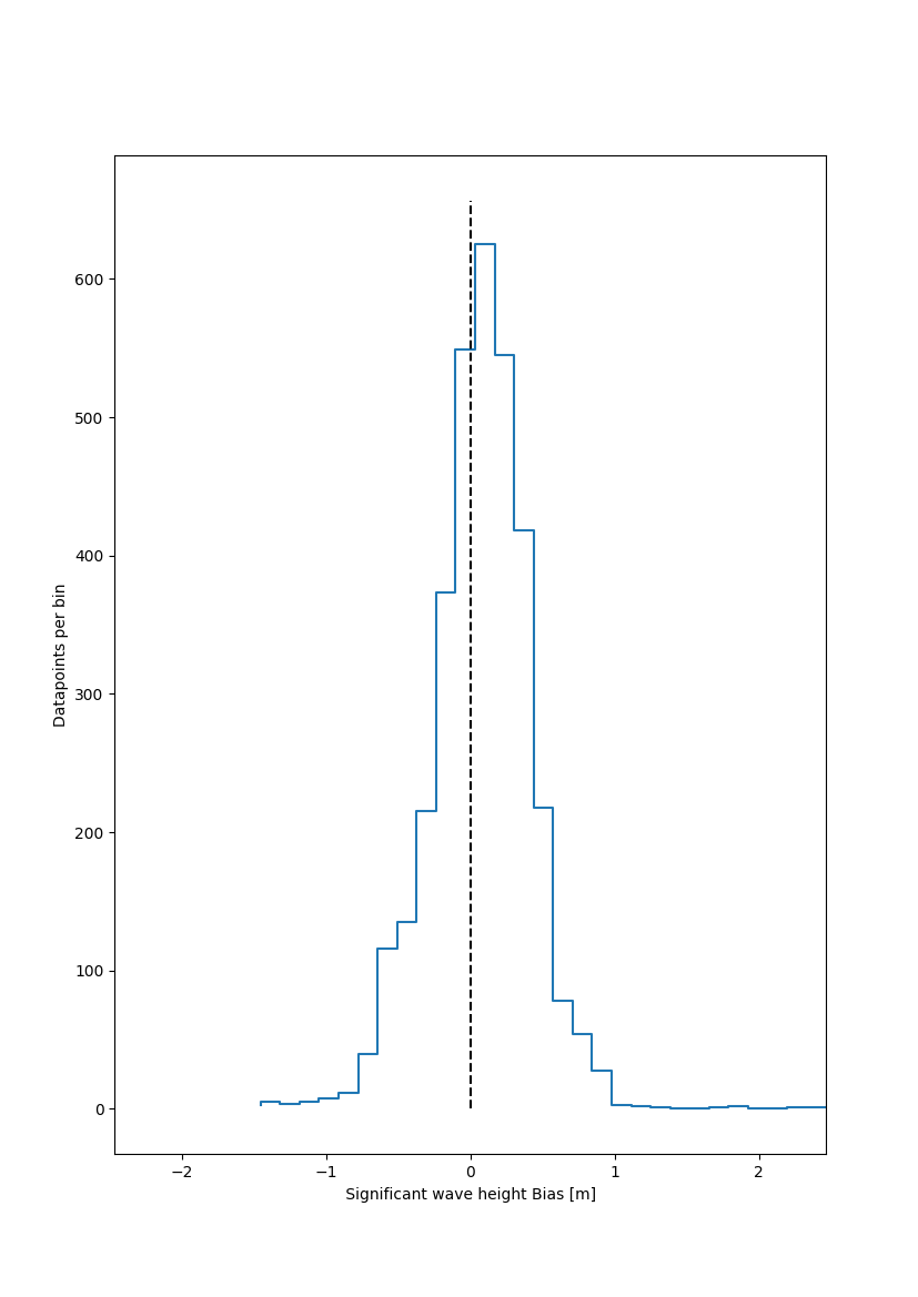
BIAS histogramm examples

import pandas as pd
import toto
import matplotlib.pyplot as plt
from toto.inputs.txt import TXTfile
import os
# read the file
hindcast='https://raw.githubusercontent.com/calypso-science/Toto/master/_tests/txt_file/tahuna_hindcast.txt'
measured='https://raw.githubusercontent.com/calypso-science/Toto/master/_tests/txt_file/tahuna_measured.txt'
os.system('wget %s ' % hindcast)
os.system('wget %s ' % measured)

me=TXTfile(['tahuna_measured.txt'],colNamesLine=1,skiprows=1,unitNamesLine=0,time_col_name={'Year':'year','Month':'month','Day':'day','Hour':'hour','Min':'Minute'})
me.reads()
me.read_time()
me=me._toDataFrame()

hd=TXTfile(['tahuna_hindcast.txt'],colNamesLine=1,skiprows=1,unitNamesLine=0,time_col_name={'Year':'year','Month':'month','Day':'day','Hour':'hour','Min':'Minute'})
hd.reads()
hd.read_time()
hd=hd._toDataFrame()



tmp=me[0].reindex(hd[0].index,method='nearest')
hd[0]['hs_measured']=tmp['Sig. Wave']
hd[0].filename='Tahuna'
# # Processing
hd[0].StatPlots.BIAS_histogramm(measured='hs_measured',modelled='hs',
        args={'Nb of bins':30,
        'Xlabel':'Significant wave height',
        'units':'m',
        'display':'On',
        })